34 广义可加模型
相比于广义线性模型,广义可加模型可以看作是一种非线性模型,模型中含有非线性的成分。
- 多元适应性(自适应)回归样条 multivariate adaptive regression splines
- Friedman, Jerome H. 1991. Multivariate Adaptive Regression Splines. The Annals of Statistics. 19(1):1–67. https://doi.org/10.1214/aos/1176347963
- earth: Multivariate Adaptive Regression Splines http://www.milbo.users.sonic.net/earth
- Friedman, Jerome H. 2001. Greedy function approximation: A gradient boosting machine. The Annals of Statistics. 29(5):1189–1232. https://doi.org/10.1214/aos/1013203451
- Friedman, Jerome H., Trevor Hastie and Robert Tibshirani. Additive Logistic Regression: A Statistical View of Boosting. The Annals of Statistics. 28(2): 337–374. http://www.jstor.org/stable/2674028
- Flexible Modeling of Alzheimer’s Disease Progression with I-Splines PDF 文档
- Implementation of B-Splines in Stan 网页文档
34.1 案例:模拟摩托车事故
34.1.1 mgcv
MASS 包的 mcycle 数据集
data(mcycle, package = "MASS")
library(ggplot2)
ggplot(data = mcycle, aes(x = times, y = accel)) +
  geom_point() +
  theme_classic() +
  labs(x = "时间(ms)", y = "加速度(g)")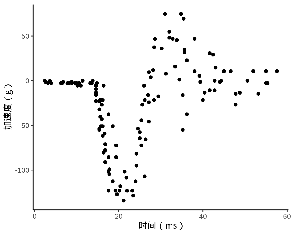
样条回归
#>
#> Family: gaussian
#> Link function: identity
#>
#> Formula:
#> accel ~ s(times)
#>
#> Parametric coefficients:
#>             Estimate Std. Error t value Pr(>|t|)
#> (Intercept)  -25.546      1.951  -13.09   <2e-16 ***
#> ---
#> Signif. codes:  0 '***' 0.001 '**' 0.01 '*' 0.05 '.' 0.1 ' ' 1
#>
#> Approximate significance of smooth terms:
#>            edf Ref.df    F p-value
#> s(times) 8.625  8.958 53.4  <2e-16 ***
#> ---
#> Signif. codes:  0 '***' 0.001 '**' 0.01 '*' 0.05 '.' 0.1 ' ' 1
#>
#> R-sq.(adj) =  0.783   Deviance explained = 79.7%
#> -REML = 616.14  Scale est. = 506.35    n = 133
方差成分
#>
#> Standard deviations and 0.95 confidence intervals:
#>
#>            std.dev     lower      upper
#> s(times) 807.88726 480.66162 1357.88215
#> scale     22.50229  19.85734   25.49954
#>
#> Rank: 2/2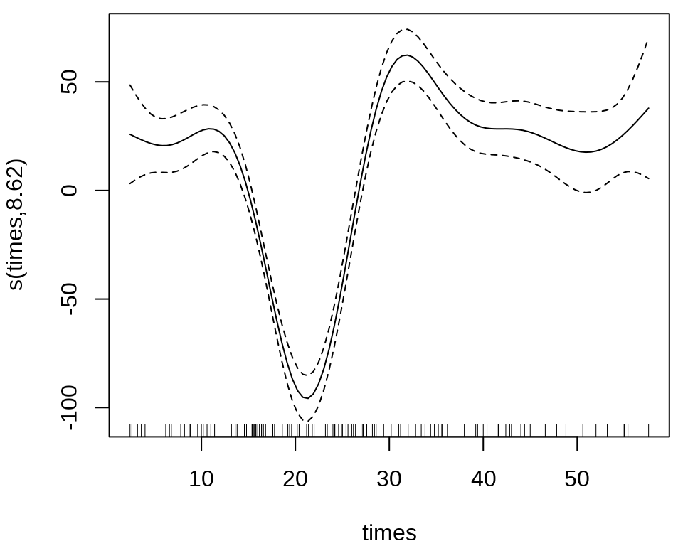
34.1.2 Stan
34.2 案例:朗格拉普岛核污染
从线性到可加,意味着从线性到非线性,可加模型容纳非线性的成分,比如高斯过程、样条。
34.2.1 mgcv
本节复用 章节 27 朗格拉普岛核污染数据,相关背景不再赘述,下面首先加载数据到 R 环境。
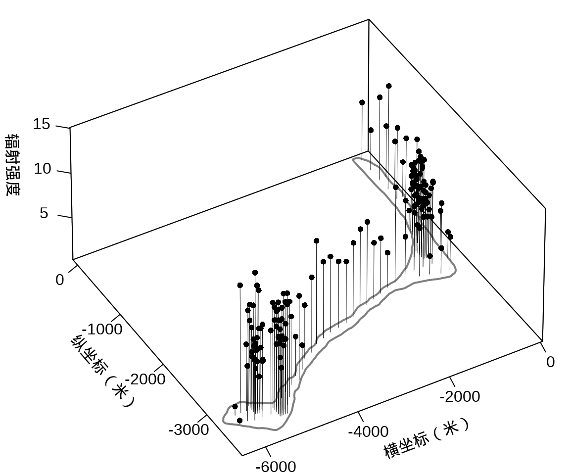
接着,将岛上各采样点的辐射强度展示出来,算是简单回顾一下数据概况。
代码
library(plot3D)
with(rongelap, {
  opar <- par(mar = c(.1, 2.5, .1, .1), no.readonly = TRUE)
  rongelap_coastline$cZ <- 0
  scatter3D(
    x = cX, y = cY, z = counts / time,
    xlim = c(-6500, 50), ylim = c(-3800, 110),
    xlab = "\n横坐标(米)", ylab = "\n纵坐标(米)",
    zlab = "\n辐射强度", lwd = 0.5, cex = 0.8,
    pch = 16, type = "h", ticktype = "detailed",
    phi = 40, theta = -30, r = 50, d = 1,
    expand = 0.5, box = TRUE, bty = "b",
    colkey = F, col = "black",
    panel.first = function(trans) {
      XY <- trans3D(
        x = rongelap_coastline$cX,
        y = rongelap_coastline$cY,
        z = rongelap_coastline$cZ,
        pmat = trans
      )
      lines(XY, col = "gray50", lwd = 2)
    }
  )
  rongelap_coastline$cZ <- NULL
  on.exit(par(opar), add = TRUE)
})
在这里,从广义可加混合效应模型的角度来对核污染数据建模,空间效应仍然是用高斯过程来表示,响应变量服从带漂移项的泊松分布。采用 mgcv 包 (Wood 2004) 的函数 gam() 拟合模型,其中,含 49 个参数的样条近似高斯过程,高斯过程的核函数为默认的梅隆型。更多详情见 mgcv 包的函数 s() 帮助文档参数的说明,默认值是梅隆型相关函数及默认的范围参数,作者自己定义了一套符号约定。
library(nlme)
library(mgcv)
fit_rongelap_gam <- gam(
  counts ~ s(cX, cY, bs = "gp", k = 50), offset = log(time),
  data = rongelap, family = poisson(link = "log")
)
# 模型输出
summary(fit_rongelap_gam)
#>
#> Family: poisson
#> Link function: log
#>
#> Formula:
#> counts ~ s(cX, cY, bs = "gp", k = 50)
#>
#> Parametric coefficients:
#> Estimate Std. Error z value Pr(>|z|)
#> (Intercept) 1.976815 0.001642 1204 <2e-16 ***
#> ---
#> Signif. codes: 0 '***' 0.001 '**' 0.01 '*' 0.05 '.' 0.1 ' ' 1
#>
#> Approximate significance of smooth terms:
#> edf Ref.df Chi.sq p-value
#> s(cX,cY) 48.98 49 34030 <2e-16 ***
#> ---
#> Signif. codes: 0 '***' 0.001 '**' 0.01 '*' 0.05 '.' 0.1 ' ' 1
#>
#> R-sq.(adj) = 0.876 Deviance explained = 60.7%
#> UBRE = 153.78 Scale est. = 1 n = 157#> s(cX,cY)
#> 2543.376值得一提的是核函数的类型和默认参数的选择,参数 m 接受一个向量, m[1] 取值为 1 至 5,分别代表球型 spherical, 幂指数 power exponential 和梅隆型 Matern with \(\kappa\) = 1.5, 2.5 or 3.5 等 5 种相关/核函数。
接下来,基于岛屿的海岸线数据划分出网格,将格点作为新的预测位置。
#> Linking to GEOS 3.11.1, GDAL 3.6.4, PROJ 9.1.1; sf_use_s2() is TRUElibrary(abind)
library(stars)
# 类型转化
rongelap_sf <- st_as_sf(rongelap, coords = c("cX", "cY"), dim = "XY")
rongelap_coastline_sf <- st_as_sf(rongelap_coastline, coords = c("cX", "cY"), dim = "XY")
rongelap_coastline_sfp <- st_cast(st_combine(st_geometry(rongelap_coastline_sf)), "POLYGON")
# 添加缓冲区
rongelap_coastline_buffer <- st_buffer(rongelap_coastline_sfp, dist = 50)
# 构造带边界约束的网格
rongelap_coastline_grid <- st_make_grid(rongelap_coastline_buffer, n = c(150, 75))
# 将 sfc 类型转化为 sf 类型
rongelap_coastline_grid <- st_as_sf(rongelap_coastline_grid)
rongelap_coastline_buffer <- st_as_sf(rongelap_coastline_buffer)
rongelap_grid <- rongelap_coastline_grid[rongelap_coastline_buffer, op = st_intersects]
# 计算网格中心点坐标
rongelap_grid_centroid <- st_centroid(rongelap_grid)
# 共计 1612 个预测点
rongelap_grid_df <- as.data.frame(st_coordinates(rongelap_grid_centroid))
colnames(rongelap_grid_df) <- c("cX", "cY")模型对象 fit_rongelap_gam 在新的格点上预测核辐射强度,接着整理预测结果数据。
# 预测
rongelap_grid_df$ypred <- as.vector(predict(fit_rongelap_gam, newdata = rongelap_grid_df, type = "response"))
# 整理预测数据
rongelap_grid_sf <- st_as_sf(rongelap_grid_df, coords = c("cX", "cY"), dim = "XY")
rongelap_grid_stars <- st_rasterize(rongelap_grid_sf, nx = 150, ny = 75)
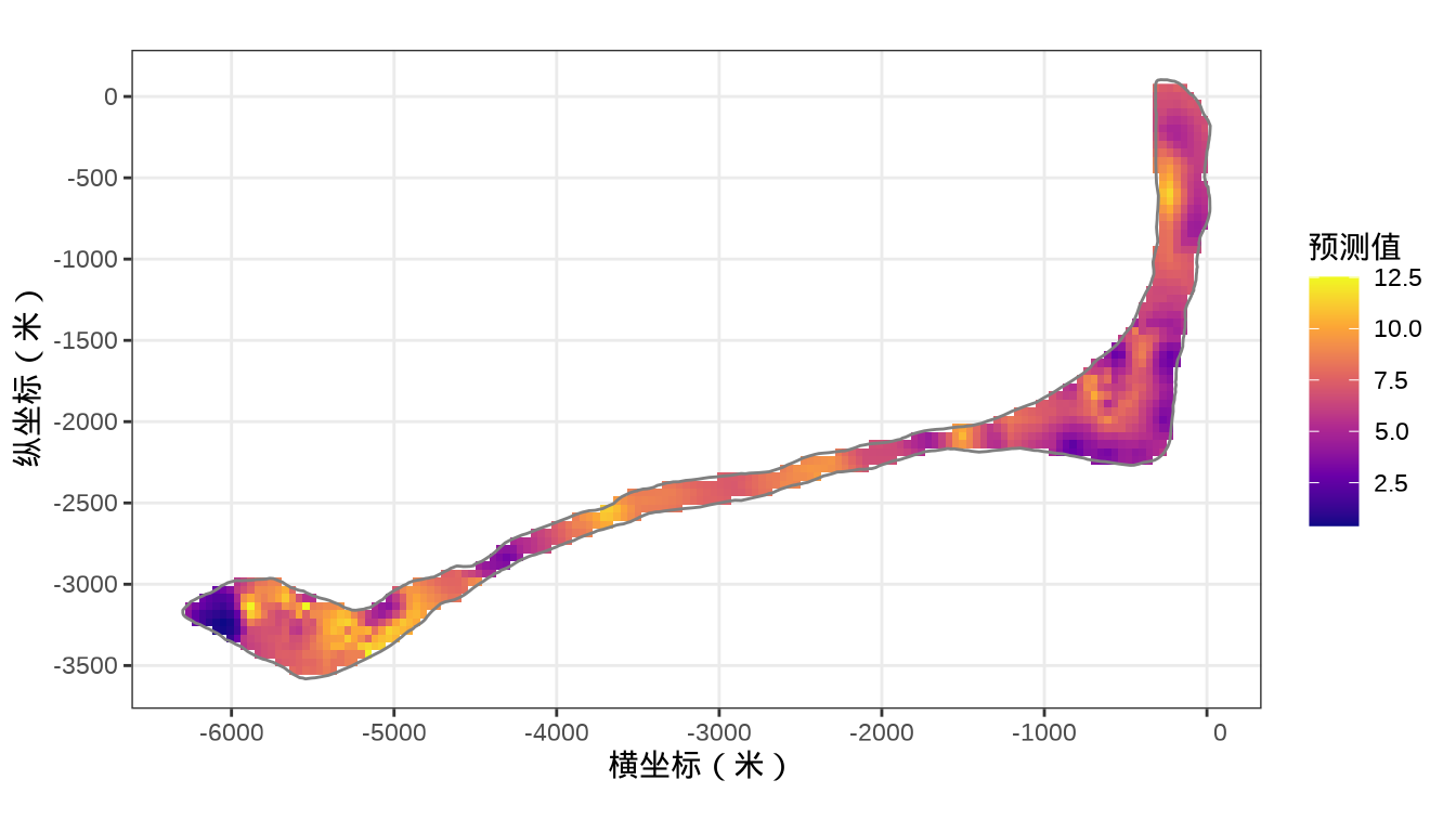
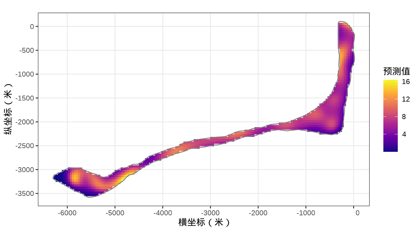
rongelap_stars <- st_crop(x = rongelap_grid_stars, y = rongelap_coastline_sfp)最后,将岛上各个格点的核辐射强度绘制出来,给出全岛核辐射强度的空间分布。
代码
代码
library(brms)
# 预计运行 1 个小时以上
rongelap_brm <- brm(counts ~ gp(cX, cY) + offset(log(time)),
  data = rongelap, family = poisson(link = "log")
)
# 5 个基函数 computing approximate GPs.
rongelap_brm <- brm(
  counts ~ gp(cX, cY, c = 5/4, k = 5) + offset(log(time)),
  data = rongelap, family = poisson(link = "log")
)
34.2.2 INLA
mgcv 包的函数 ginla() 实现简化版的 Integrated Nested Laplace Approximation, INLA (Rue, Martino, 和 Chopin 2009)。
rongelap_gam <- gam(
  counts ~ s(cX, cY, bs = "gp", k = 50), offset = log(time),
  data = rongelap, family = poisson(link = "log"), fit = FALSE
)
# 简化版 INLA
fit_rongelap_ginla <- ginla(G = rongelap_gam)
str(fit_rongelap_ginla)
#> List of 2
#> $ density: num [1:50, 1:100] 2.49e-01 9.03e-06 3.51e-06 1.97e-06 1.17e-06 ...
#> $ beta : num [1:50, 1:100] 1.97 -676.61 -572.67 4720.77 240.12 ...其中, \(k = 50\) 表示 49 个样条参数,每个参数的分布对应有 100 个采样点,另外,截距项的边际后验概率密度分布如下:
plot(
  fit_rongelap_ginla$beta[1, ], fit_rongelap_ginla$density[1, ],
  type = "l", xlab = "截距项", ylab = "概率密度"
)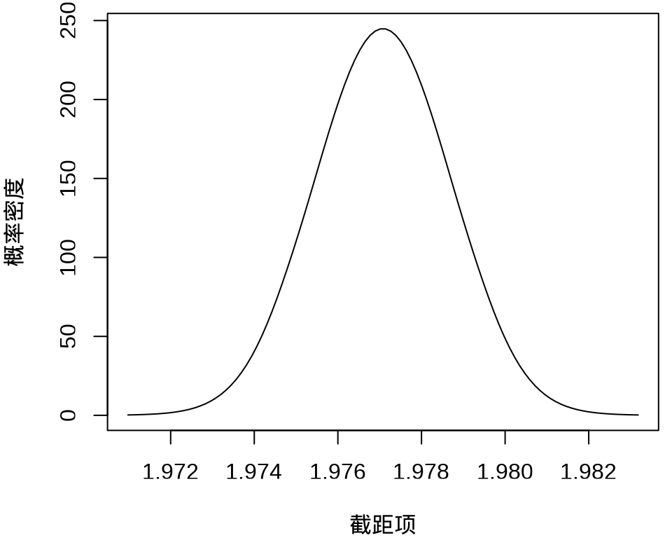
不难看出,截距项在 1.976 至 1.978 之间,50个参数的最大后验估计分别如下:
idx <- apply(fit_rongelap_ginla$density, 1, function(x) x == max(x))
fit_rongelap_ginla$beta[t(idx)]
#> [1] 1.977019e+00 -5.124099e+02 5.461183e+03 1.515296e+03 -2.822166e+03
#> [6] -1.598371e+04 -6.417855e+03 1.938122e+02 -4.270878e+03 3.769951e+03
#> [11] -1.002035e+04 1.914717e+03 -9.721572e+03 -3.794461e+04 -1.401549e+04
#> [16] -5.376582e+04 -1.585899e+04 -2.338235e+04 6.239053e+04 -3.574501e+02
#> [21] -4.587927e+04 1.723604e+04 -4.514781e+03 9.184026e-02 3.496526e-01
#> [26] -1.477406e+02 4.585057e+03 9.153647e+03 1.929387e+04 -1.116512e+04
#> [31] -1.166149e+04 8.079451e+02 3.627369e+03 -9.835680e+03 1.357777e+04
#> [36] 1.487742e+04 3.880562e+04 -1.708858e+03 2.775844e+04 2.527415e+04
#> [41] -3.932957e+04 3.548123e+04 -1.116341e+04 1.630910e+04 -9.789381e+02
#> [46] -2.011250e+04 2.699657e+04 -4.744393e+04 2.753347e+04 2.834356e+04接下来,介绍完整版的近似贝叶斯推断方法 INLA — 集成嵌套拉普拉斯近似 (Integrated Nested Laplace Approximations,简称 INLA) (Rue, Martino, 和 Chopin 2009)。根据研究区域的边界构造非凸的内外边界,处理边界效应。
library(INLA)
library(splancs)
# 构造非凸的边界
boundary <- list(
  inla.nonconvex.hull(
    points = as.matrix(rongelap_coastline[,c("cX", "cY")]),
    convex = 100, concave = 150, resolution = 100),
  inla.nonconvex.hull(
    points = as.matrix(rongelap_coastline[,c("cX", "cY")]),
    convex = 200, concave = 200, resolution = 200)
)
根据研究区域的情况构造网格,边界内部三角网格最大边长为 300,边界外部最大边长为 600,边界外凸出距离为 100 米。
构建 SPDE,指定自协方差函数为指数型,则 \(\nu = 1/2\) ,因是二维平面,则 \(d = 2\) ,根据 \(\alpha = \nu + d/2\) ,从而 alpha = 3/2 。
生成 SPDE 模型的指标集,也是随机效应部分。
#>       s s.group  s.repl
#>     691     691     691
投影矩阵,三角网格和采样点坐标之间的投影。观测数据 rongelap 和未采样待预测的位置数据 rongelap_grid_df
# 观测位置投影到三角网格上
A <- inla.spde.make.A(mesh = mesh, loc = as.matrix(rongelap[, c("cX", "cY")]) )
# 预测位置投影到三角网格上
coop <- as.matrix(rongelap_grid_df[, c("cX", "cY")])
Ap <- inla.spde.make.A(mesh = mesh, loc = coop)
# 1612 个预测位置
dim(Ap)
#> [1] 1612 691准备观测数据和预测位置,构造一个 INLA 可以使用的数据栈 Data Stack。
# 在采样点的位置上估计 estimation stk.e
stk.e <- inla.stack(
  tag = "est",
  data = list(y = rongelap$counts, E = rongelap$time),
  A = list(rep(1, 157), A),
  effects = list(data.frame(b0 = 1), s = indexs)
)

# 在新生成的位置上预测 prediction stk.p
stk.p <- inla.stack(
  tag = "pred",
  data = list(y = NA, E = NA),
  A = list(rep(1, 1612), Ap),
  effects = list(data.frame(b0 = 1), s = indexs)
)

# 合并数据 stk.full has stk.e and stk.p
stk.full <- inla.stack(stk.e, stk.p)
指定响应变量与漂移项、联系函数、模型公式。
# 模型拟合
res <- inla(formula = y ~ 0 + b0 + f(s, model = spde),
  data = inla.stack.data(stk.full),
  E = E, # E 已知漂移项
  control.family = list(link = "log"),
  control.predictor = list(
    compute = TRUE,
    link = 1, # 与 control.family 联系函数相同
    A = inla.stack.A(stk.full)
  ),
  control.compute = list(
    cpo = TRUE,
    waic = TRUE, # WAIC 统计量 通用信息准则
    dic = TRUE   # DIC 统计量 偏差信息准则
  ),
  family = "poisson"
)
# 模型输出
summary(res)
#>
#> Call:
#> c("inla.core(formula = formula, family = family, contrasts = contrasts,
#> ", " data = data, quantiles = quantiles, E = E, offset = offset, ", "
#> scale = scale, weights = weights, Ntrials = Ntrials, strata = strata,
#> ", " lp.scale = lp.scale, link.covariates = link.covariates, verbose =
#> verbose, ", " lincomb = lincomb, selection = selection, control.compute
#> = control.compute, ", " control.predictor = control.predictor,
#> control.family = control.family, ", " control.inla = control.inla,
#> control.fixed = control.fixed, ", " control.mode = control.mode,
#> control.expert = control.expert, ", " control.hazard = control.hazard,
#> control.lincomb = control.lincomb, ", " control.update =
#> control.update, control.lp.scale = control.lp.scale, ", "
#> control.pardiso = control.pardiso, only.hyperparam = only.hyperparam,
#> ", " inla.call = inla.call, inla.arg = inla.arg, num.threads =
#> num.threads, ", " keep = keep, working.directory = working.directory,
#> silent = silent, ", " inla.mode = inla.mode, safe = FALSE, debug =
#> debug, .parent.frame = .parent.frame)" )
#> Time used:
#> Pre = 1.06, Running = 2.05, Post = 0.0868, Total = 3.2
#> Fixed effects:
#> mean sd 0.025quant 0.5quant 0.975quant mode kld
#> b0 1.828 0.061 1.706 1.828 1.948 1.828 0
#>
#> Random effects:
#> Name Model
#> s SPDE2 model
#>
#> Model hyperparameters:
#> mean sd 0.025quant 0.5quant 0.975quant mode
#> Theta1 for s 2.00 0.063 1.88 2.00 2.12 2.00
#> Theta2 for s -4.85 0.130 -5.11 -4.85 -4.59 -4.85
#>
#> Deviance Information Criterion (DIC) ...............: 1834.56
#> Deviance Information Criterion (DIC, saturated) ....: 314.90
#> Effective number of parameters .....................: 156.46
#>
#> Watanabe-Akaike information criterion (WAIC) ...: 1789.31
#> Effective number of parameters .................: 80.06
#>
#> Marginal log-Likelihood: -1331.95
#> CPO, PIT is computed
#> Posterior summaries for the linear predictor and the fitted values are computed
#> (Posterior marginals needs also 'control.compute=list(return.marginals.predictor=TRUE)')kld表示 Kullback-Leibler divergence (KLD) 它的值描述标准高斯分布与 Simplified Laplace Approximation 之间的差别,值越小越表示拉普拉斯的近似效果好。DIC 和 WAIC 指标都是评估模型预测表现的。另外,还有两个量计算出来了,但是没有显示,分别是 CPO 和 PIT 。CPO 表示 Conditional Predictive Ordinate (CPO),PIT 表示 Probability Integral Transforms (PIT) 。
固定效应(截距)和超参数部分
#>        mean         sd 0.025quant 0.5quant 0.975quant     mode          kld
#> b0 1.828057 0.06149191 1.706415 1.828314 1.948234 1.828309 1.782796e-08#> mean sd 0.025quant 0.5quant 0.975quant mode
#> Theta1 for s 2.000465 0.06252212 1.876613 2.000728 2.122784 2.001823
#> Theta2 for s -4.851576 0.12998467 -5.106817 -4.851802 -4.595020 -4.852739提取预测数据,并整理数据。
# 预测值对应的指标集合
index <- inla.stack.index(stk.full, tag = "pred")$data
# 提取预测结果,后验均值
# pred_mean <- res$summary.fitted.values[index, "mean"]
# 95% 预测下限
# pred_ll <- res$summary.fitted.values[index, "0.025quant"]
# 95% 预测上限
# pred_ul <- res$summary.fitted.values[index, "0.975quant"]
# 整理数据
rongelap_grid_df$ypred <- res$summary.fitted.values[index, "mean"]
# 预测值数据
rongelap_grid_sf <- st_as_sf(rongelap_grid_df, coords = c("cX", "cY"), dim = "XY")
rongelap_grid_stars <- st_rasterize(rongelap_grid_sf, nx = 150, ny = 75)
rongelap_stars <- st_crop(x = rongelap_grid_stars, y = rongelap_coastline_sfp)
最后,类似之前 mgcv 建模的最后一步,将 INLA 的预测结果绘制出来。